- Canonical plane
- Stereotaxic topography
- Arbitrary plane
- Automatic registration
- Data sharing
- Atlas mapping
- Virtual surgery
- Atlas Reslicing
- Neuronal Circuits
- FAQ
Manual Instruction
Canonical plane visualization


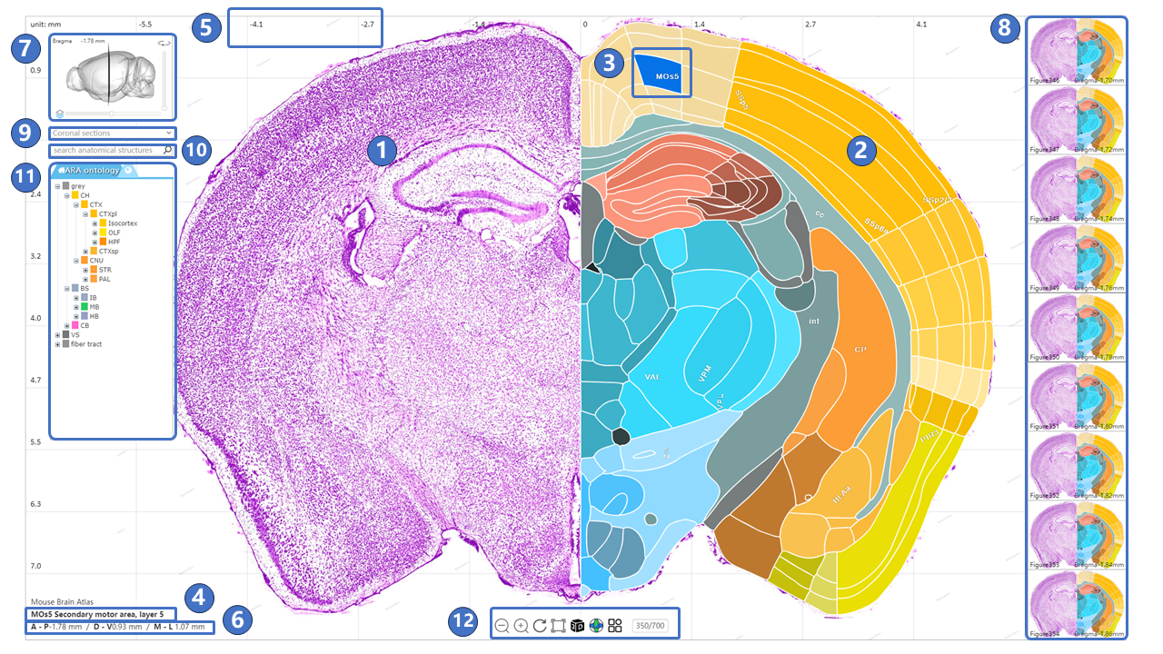
The interface for the canonical plane visualization service is illustrated below. The central area is the main window, used to display STAM's canonical planes (①) and the brain region annotations on these planes (②). Users can use the left mouse button and scroll wheel in the main window to move, and zoom in to the resolution of the region of interest. When the user hovers the mouse over an annotation for a brain region or nucleus, the annotation switches to a blue highlighted mode (③), and the full name of the highlighted brain region or nucleus is displayed in the lower-left corner (④). The light gray grid behind the canonical plane and annotations shows the distribution of the STAM coordinate system on the current plane (⑤). As the user moves the mouse, the real-time position of the mouse in the STAM coordinate system is displayed in the lower-left corner of the main window (⑥). Users can also observe the position of the current viewed canonical plane in the entire mouse brain through the navigation window in the upper left corner (⑦), as well as drag the slide inside the navigation window in the upper left corner to jump to other canonical planes of interest. Users can freely switch to other sections using the right-side image gallery (⑧), or switch between different anatomical directions, such as coronal, sagittal, and horizontal planes (⑨). Additionally, users can search for brain regions or nuclei of interest in the input box (⑩) or navigate through the anatomical ontology tree (⑪). If the current viewed profile does not include the searched structure, it will jump to the nearest profile in the same direction that contains the structure. At the bottom of the main window is the button panel for the canonical plane visualization service (⑫). The button functions, from left to right, include: Home, zoom out, zoom in, reset view, full screen, switch to three-dimensional visualization service,downloading, switch to arbitrary angle cross-section visualization service, display mode switch,guide,feedback, QR code and jump to other profiles in the current anatomical direction. To input the numerical designation of a coronal plane into the text input box in the button group, then press the enter key on the keyboard to jump to the corresponding plane. The viewing perspective, i.e., the current zoom level and position, will be preserved when switching between planes. Furthermore, we could traverse from canonical plane visualization service to stereotaxic topography visualization service: On the canonical plane visualization service page, users can highlight a brain region or nucleus of interest, then click the 3D button in the button panel at the bottom of the page, or right-click and choose to jump to the stereotaxic topography visualization service page from the pop-up menu. The brain region or nucleus highlighted in the canonical plane visualization page will also display its three-dimensional model in the stereotaxic topography visualization page.
Stereotaxic topography visualization
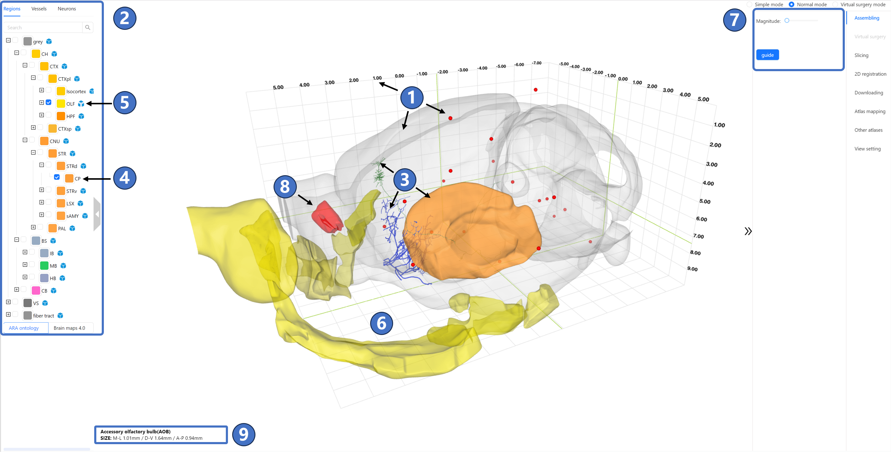
The stereotactic topography service interface is shown in the figure. The central area is the main window. The three arrows labeled by (①) indicate the semi-transparent outline of the mouse brain, a three-dimensional coordinate system displayed in numerical grid, and the cranial and intracranial datum marks shown as red dots. The primary purpose of this information is to provide users with intuitive and diverse forms of spatial localization information, all of which are displayed by default upon entering the service interface. On the left of the main window is the data panel (②), which contains three tabs. The “Regions“ tab includes the anatomical nomenclature tree of STAM, where users can select any number of structures of interest via checkboxes. The “Neurons“ tab is used to query and filter neuron morphological data with somas or projection targets located in regions of interest. Data selected or filtered in these three tabs will be displayed in the main window. As shown by the two arrows labeled (③), the orange represents the three-dimensional topography of the brain regions of interest selected in the “Regions“ tab (④), and the green represents the individual neuron morphological data filtered in the “Neurons“ tab. In the anatomical nomenclature tree under the “Regions“ tab, a blue square icon could be found at the right side of any brain region or nucleus that consists of substructures. As shown in (⑤), when users click on this icon next to the structure of interest, the original blue square changes to an icon composed of three expanded surfaces. At this point, all substructures of the clicked structure will be visualized in an assembled form in the main window, as indicated by the golden three-dimensional models in (⑥). When the Assembling tab be selected, all substructures will expand from their original positions, and the expansion magnitude can be set in the right panel (⑦). When three-dimensional models of brain regions or nuclei have been loaded in the main window, users can move the mouse over any model of interest, causing its color to change to red, as shown by (⑧). At this time, detailed information about the structure, including its full name, abbreviation, and three-dimensional size, will appear in the lower left corner of the main window, as shown by (⑨). At the bottom of the main window is the button panel for the canonical plane visualization service (⑩). The button functions, from left to right, include: Home,Coronal view, Sagittal view, Horizontal view, Reset the focus, Setting, Feedback.
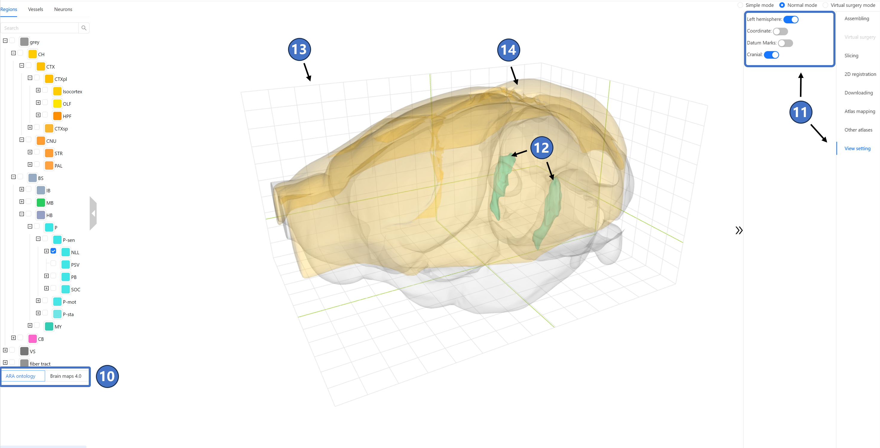
Furthermore, if users would like to modify the default display options provided by STAM, they can switch to the “View setting“ tab on the right, which contains four toggle options (⑪). The “Left hemisphere“ switch determines whether the left hemisphere is displayed in the main window, and it is off by default. When this option is set to “On,“ any anatomical structure will be displayed in both hemispheres simultaneously, as shown in (⑫). The “Coordinate“ switch determines whether coordinate values are displayed in the main window, and it is on by default, as shown in (⑬). When set to “Off,“ only the grid is displayed in the main window. The “Datum Marks“ switch determines whether datum marks are displayed in the main window, and it is on by default, as shown in (⑭). When set to “Off,“ the 20 datum marks marked by red spheres will no longer be displayed in the main window. The “Cranial“ switch determines whether the three-dimensional contour of the skull is displayed in the main window, and it is off by default. When set to “On,“ a light blue skull model appears in the main window, which includes only the partial area located directly above the mouse brain, not the complete skull, as shown in (⑮). The Grid switch determines whether to display the grid in the main window, with the default being On, as shown in (⑯). The Terminals switch determines whether to display the terminals of neurons in the main window, default is On. The Branchings switch determines whether to display the branching points of neurons in the main window, default is On. The Brain contour switch determines whether to display the extracranial contour in the main window, default is On, as shown in (⑰). Lastly, the coordinate system is shared across all STAM services, including the stereotaxic topography visualization service. By default, this coordinate system uses the Bregma point as the origin. Users can also switch the coordinate origin to any of the other 19 cranial or intracranial datum marks provided by STAM, and the coordinates of the objects visualized in the main window will be recalculated based on the new origin.
Arbitrary plane visualization
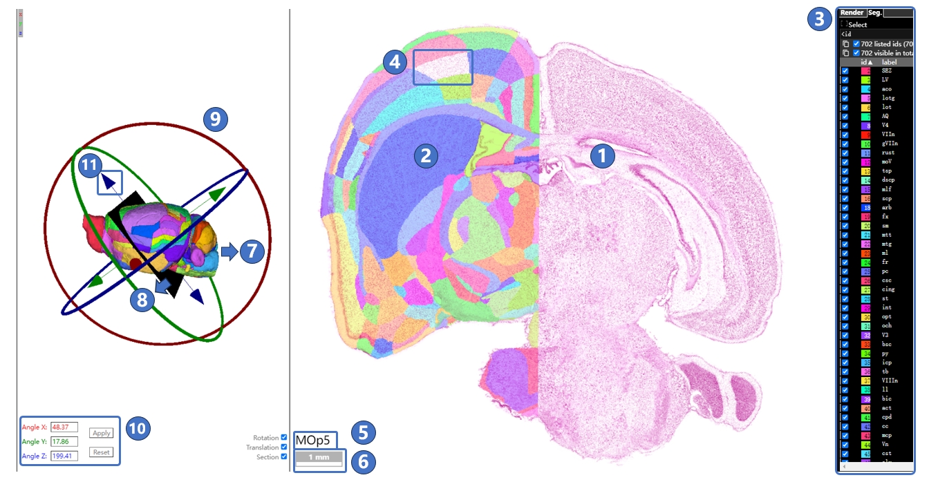
The interface for the Arbitrary plane visualization is illustrated as followed. The left side features the navigation window, while the right side is the main window. The main window displays the arbitrary angle slice of STAM (①) and the brain region annotations on that slice (②). Users can pan in the main window by holding down the left mouse button, zoom in using Ctrl + scroll wheel, or switch to different neighboring slices along the current angle by using the scroll wheel. On the right side of the main window is the list of brain regions and nuclei (③). When the user moves the mouse over the name of a structure of interest, the annotation for that structure in the main window is highlighted in light gray (④). Users can also move the mouse over the annotation of a structure of interest in the main window, and the name of that structure in the list of brain regions and nuclei on the right will automatically be highlighted. At this time, the name of the structure will also be displayed in the lower-left corner of the main window (⑤). Below the structure name is the scale bar of the slice image in the main window at the current resolution (⑥). In the navigation window on the left side, the central area displays the three-dimensional model of the right half of the mouse brain (⑦). The black plane corresponds to the position and angle of the slice in the main window (⑧). The red, green, and blue circles around the model are used to change the pitching, rotation, and rolling angles of the cross-section (⑨). Users can also input values in the lower-left corner of the navigation window to set the slice angle (⑩). The red, green, and blue arrows in the navigation window are used to determine the position of the slice along the given arbitrary angle in the three-dimensional space (⑪).
Automatic slice registration
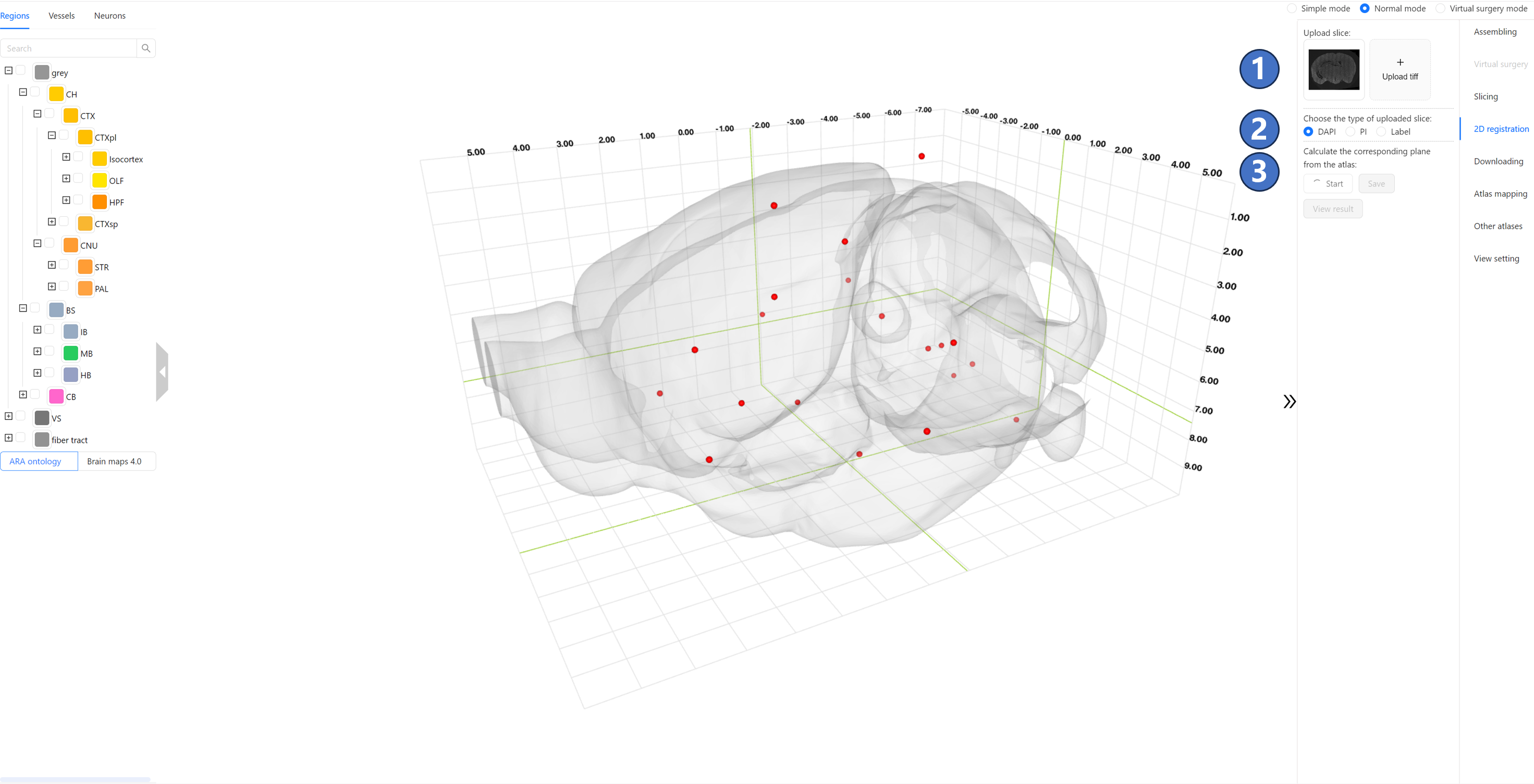
Operating Instructions The interface for the brain slice automatic registration service is shown in the figure below. Locate the “Upload Slice“ button group ① on the right side, and click the “Upload tiff“ button to upload the 2D brain slice image in tif/tiff format for registration from your local device. (Optional) Upload the second slice, which is previously co-registered to the first uploaded slice. The uploaded image must be a mouse brain slice sampled at a resolution of 10 micrometers; slices with a resolution of 1 micrometer cannot be processed due to their large size. Currently, only PI, DAPI, and Label images are supported. Next, click the “Start“ button in the “Calculate the corresponding plane from the atlas“ button group ② and wait for the result from the server. During the calculation process, the “Start“ button will be disabled, so please be patient.
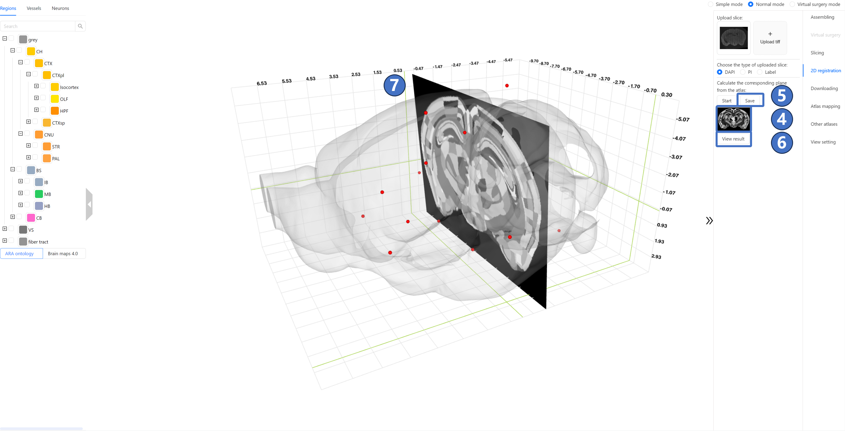
Once the calculation is complete, the “Start“ button will become available again. At this point, a preview image of the calculation result will appear below the “Start“ button ③, which can be enlarged by left-clicking. The “Save“ button ④ to the right of the “Start“ button will also become clickable. By clicking this “Save“ button, users can download the calculation result to their local device. Additionally, users can click the “View result“ button ⑤ below the preview image to display the calculation result in the main window, as shown in ⑥.Users can also check the fliplr option ⑦ on the right side of the slice, and then click on the single option first ⑧. The image in the main window will flip and display.
Data sharing
Operating Instructions The data sharing service interface is shown in the figure below. The right panel contains a “Select the range“ button ①:
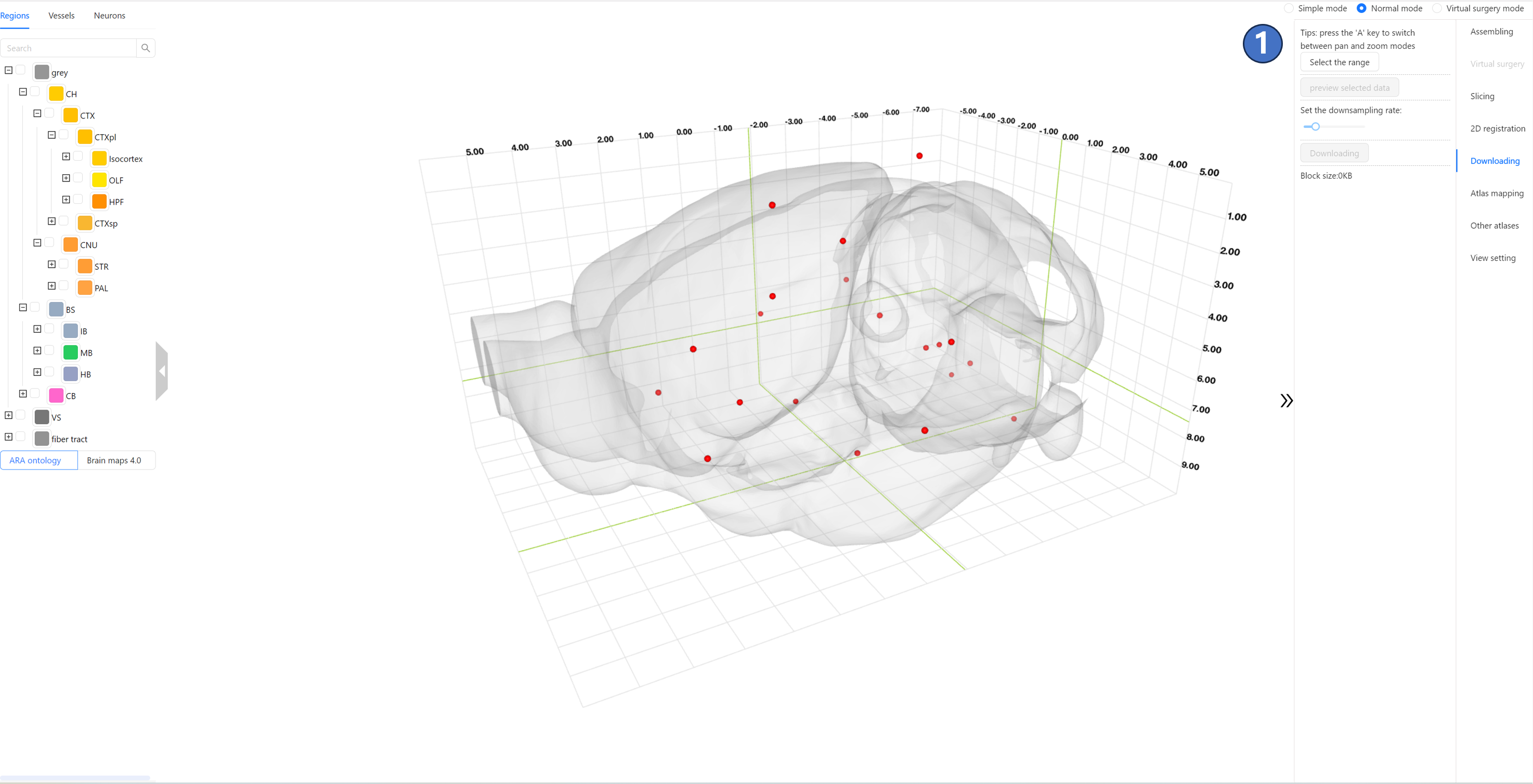
After clicking “Select the range” button, an orange-lined box ② will appear in the main window, representing the spatial range of the data to be downloaded. The top-left and bottom-right corners of the box display two sets of coordinates, indicating the range of the selected box in the current coordinate system.As shown by ③, users can control the box's translation along the X (M-L), Y (D-V), and Z (A-P) axes by left-clicking and dragging the red, green, and blue arrows, respectively. When an arrow is selected, it will be highlighted as bright yellow. Additionally, as indicated by ④, users can switch from translation mode to scaling mode by pressing the “A“ key on the keyboard. In this mode, the arrows will change to squares, as shown by ⑤, and dragging these squares will resize the box. Once the spatial range for the data to be downloaded is determined, users can click the “preview selected data“ button ⑥. This will visualize the images within the selected range in the main window using volume rendering, as shown by ⑦.
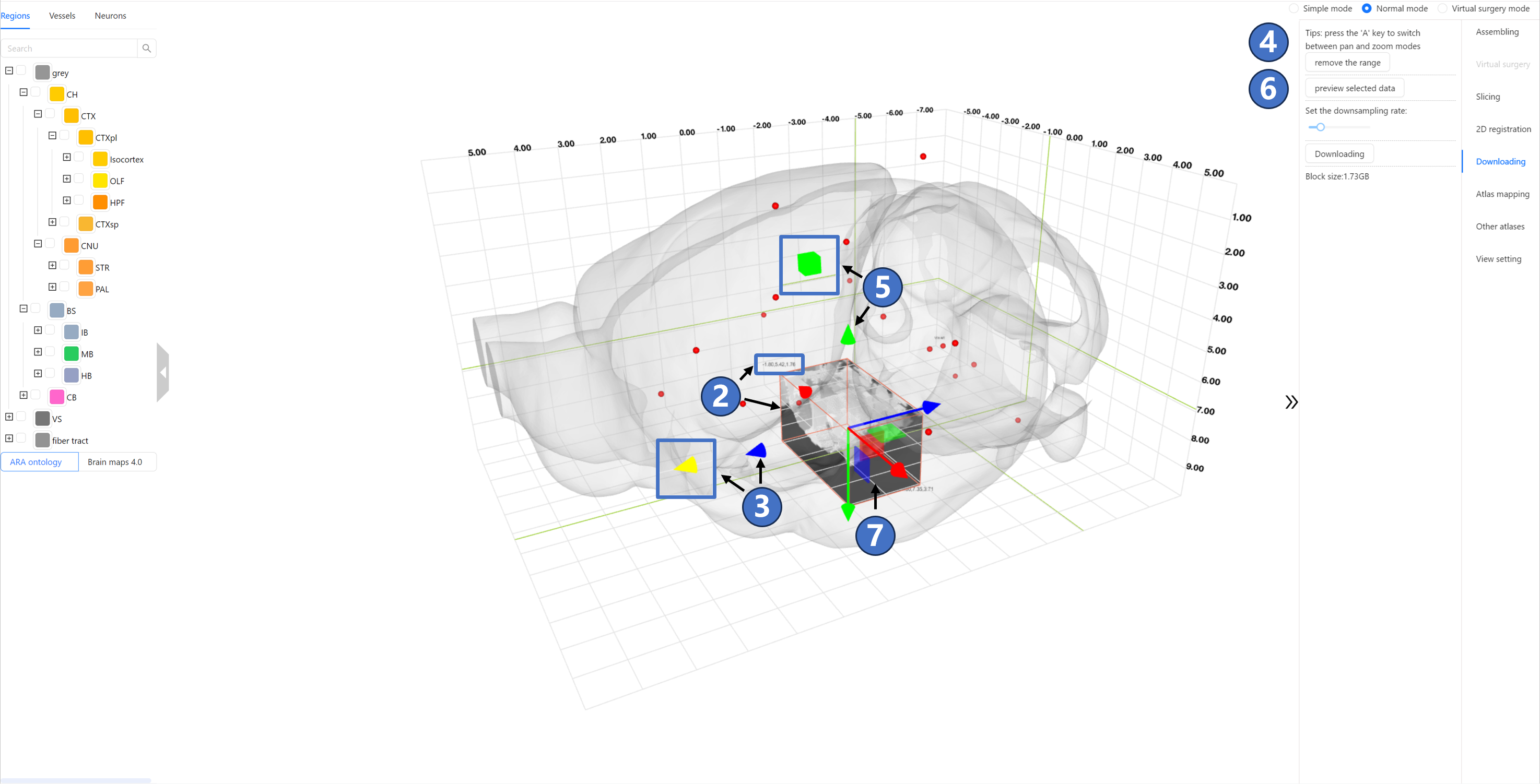
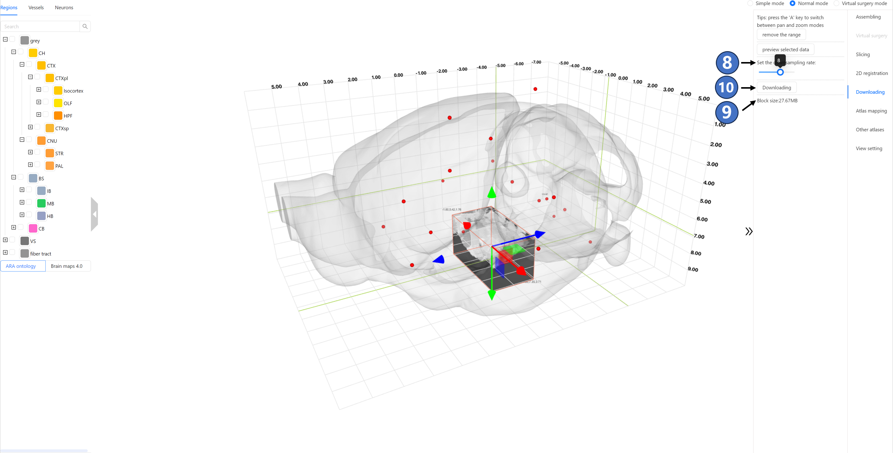
By dragging the “Set the downsampling rate“ slider, users can select the sampling rate for the data to be downloaded. The specific sampling rate value can be seen in the black-backgrounded tip above the slider. As shown by ⑧, the currently selected download data is downsampled by a factor of 2, resulting in an uncompressed data size of 1.93GB, as indicated by ⑨. If the data size does not exceed 1 GB, clicking the “Downloading“ button ⑩ will directly download the data. If the data size exceeds this limit, clicking the “Downloading“ button will invoke the user's email client (such as Outlook) and automatically fill in the email body with the selected download range and sampling rate information. By clicking the send button, users can submit a data download request to the STAM website.
Atlas mapping
Operating Instructions As shown in the figure, users can click the “Upload“ button ① in the right panel to upload 3D image data or neuronal morphology data that has been previously registered to either the CCF or STAM. The image format must be TIFF, and the neuronal morphology data format must be SWC, with a spatial resolution of 10 micrometers. After the uploading is completed, there would be an image on the left side of the “Upload“ button. Select the direction of conversion (either from STAM to CCF or vice versa) in the “Select the direction of conversion“ radio button ③. Then, click the “Start“ button ④ to start the calculation on the STAM server. At this point, the “Start“ button enters the waiting status ⑤.
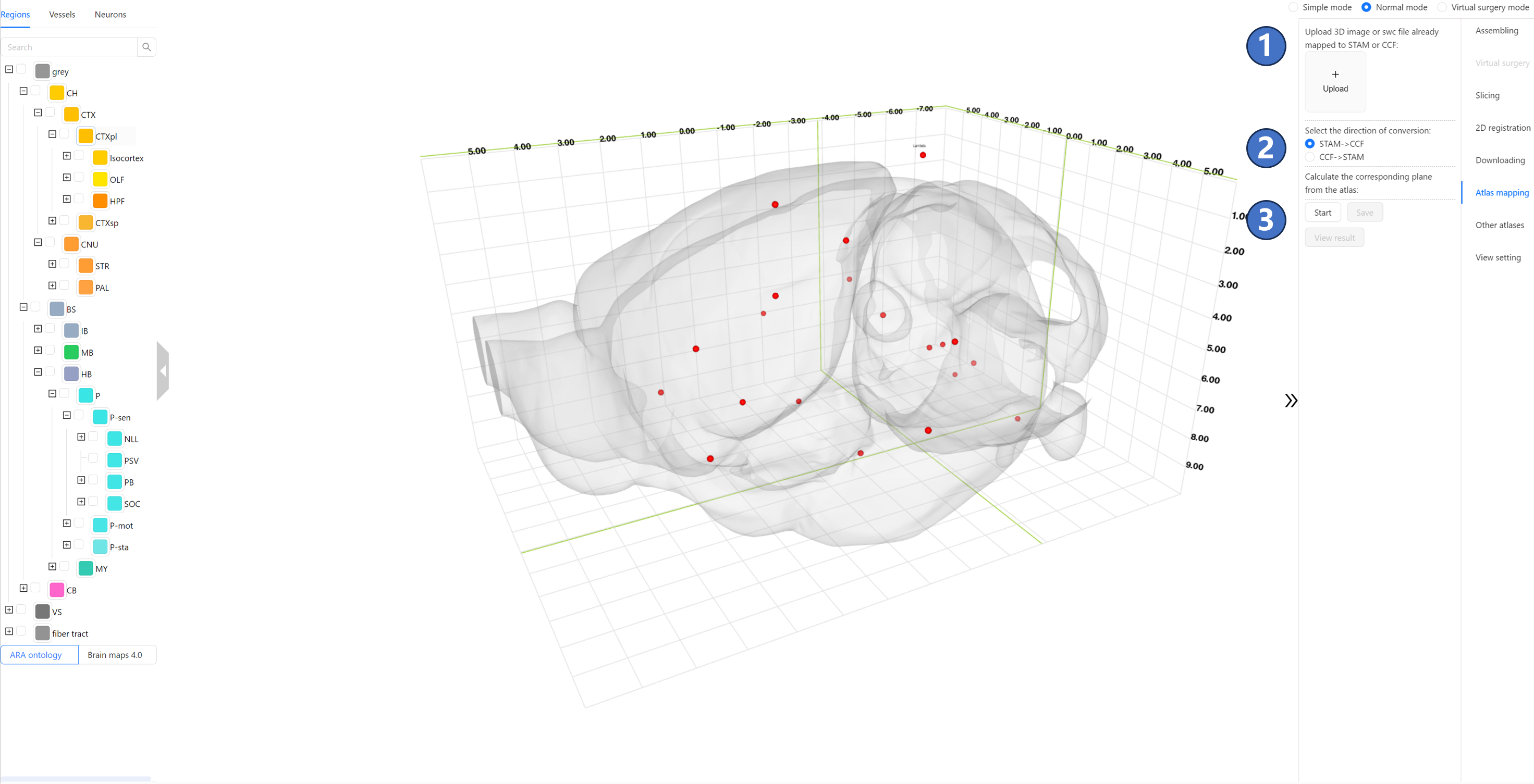
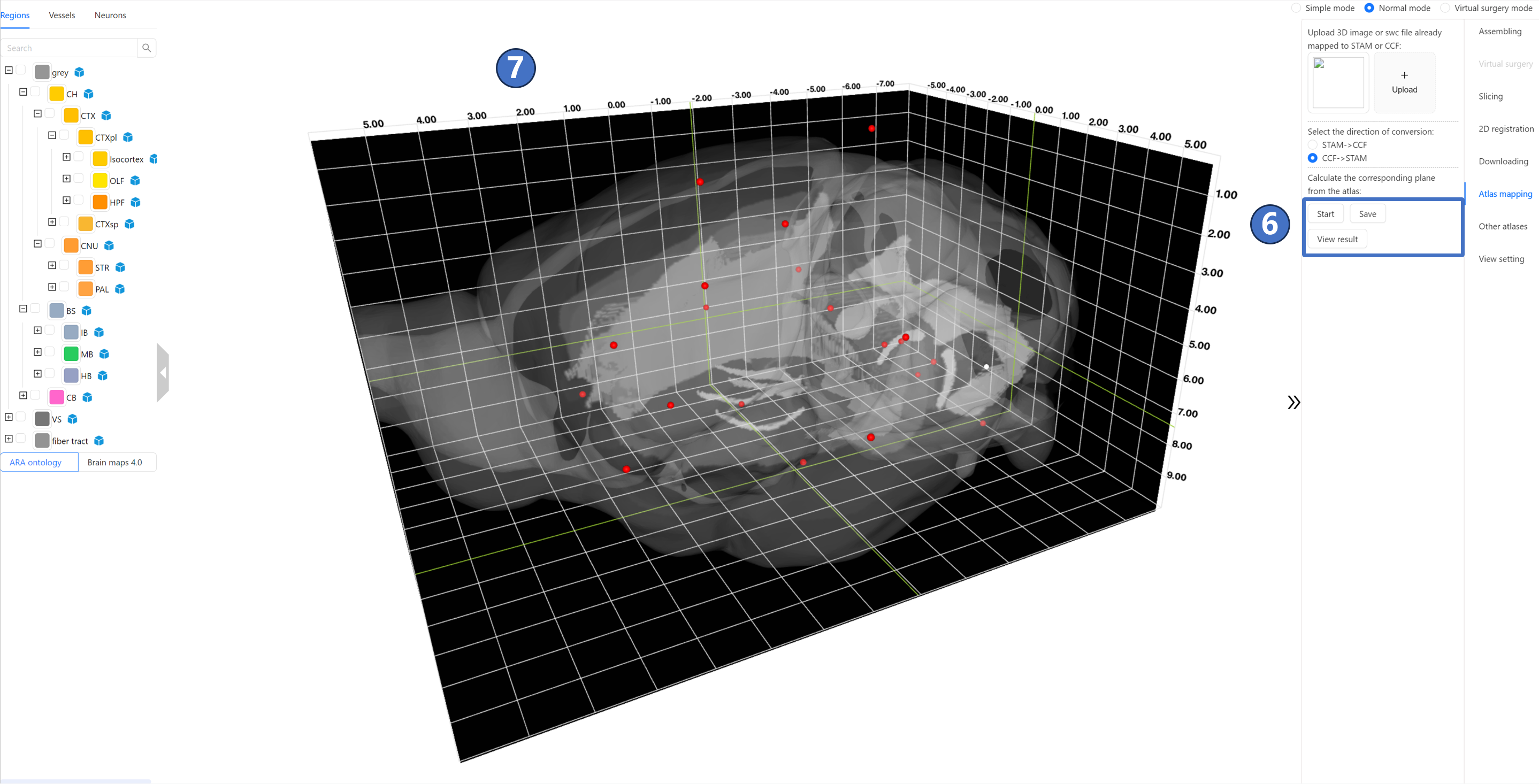
After waiting for about 10 minutes, the STAM server finishes the calculation and returns the results. At this point, both the “Save“ button and the “View result“ button become clickable ⑥. Clicking the “Save“ button allows you to download the results to your local device; clicking the “View result“ button lets you preview the calculation results in the main window ⑦.
Virtual surgery
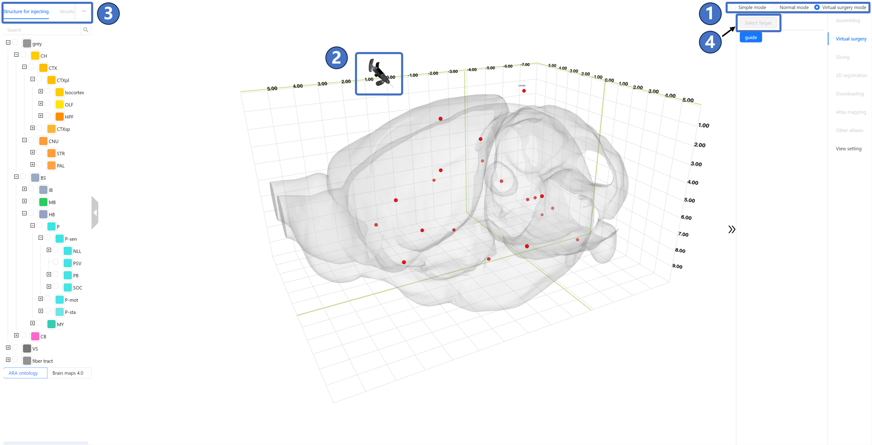
Introduction We have developed a virtual surgery navigating service. Users can simulate the stereotaxic surgical procedure of injecting viruses into the mouse brain through interactive operations. Based on user inputs, the STAM provides the information on the distance and injection angle between the injection site and origin defined by cranial or intracranial datum marks. Additionally, we offer the intelligent injection path planning: users can specify brain regions they wish to avoid, and the service will automatically calculate an appropriate path. If no suitable path can be found, the service will also give a notification. Operating Instructions The virtual surgery service is shown in the figure below. At this point, the main window is in Virtual surgery mode ①, and only the Virtual surgery is available on the right side of the page. Firstly, select the brain region for injection. Upon entering Virtual surgery mode, the mouse pointer changes to a virtual injection needle model, as shown by ②, and the “Regions” tab on the left data panel transforms into the “Structure for injecting” tab ③. Here, users need to choose a brain region for injection. Once selected, the “Select target“ button ④ highlighted in the figure becomes clickable.
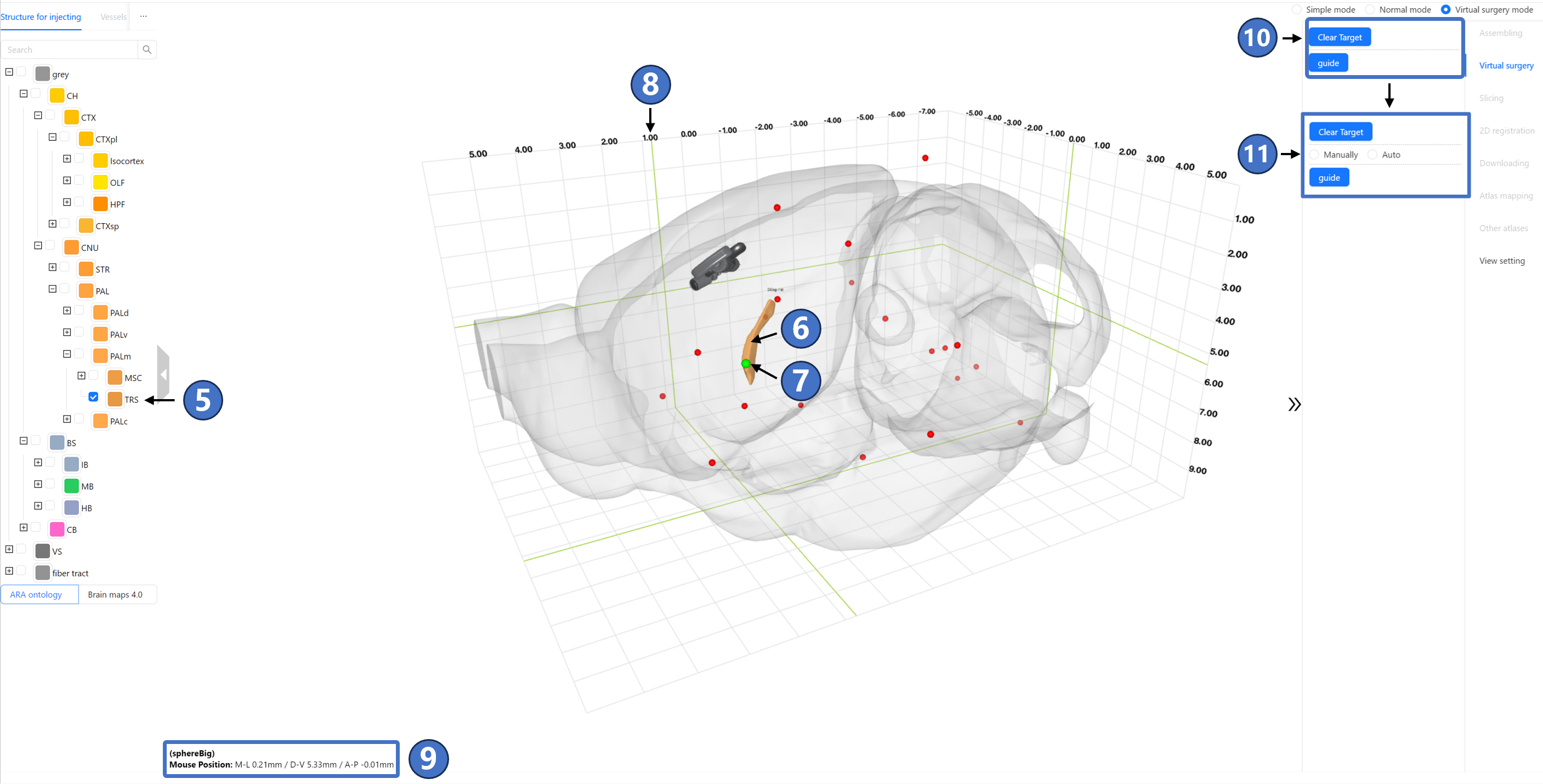
Next, select the injection target on the chosen brain region. At this point, the user has already selected a brain region for injection on the left data panel ⑤, and its 3D model ⑥ is visualized in the main window. Continuing to click the “Select target“ button, a green dot ⑦ follows the mouse cursor on the surface of the brain region's 3D model. The position of this dot is projected onto the coordinate grid of the 3D space and marked with a green crosshair ⑧. The coordinates of this point in all three directions can also be viewed in the bottom-left corner ⑨. Once the user identifies a suitable target location, they can left-click to mark it. At this point, the status on the right panel changes from ⑩ to ⑪, adding a radio button. If the user is unsatisfied with the marked location, they can click the “Clear target“ button on the panel to re-mark the injection target.
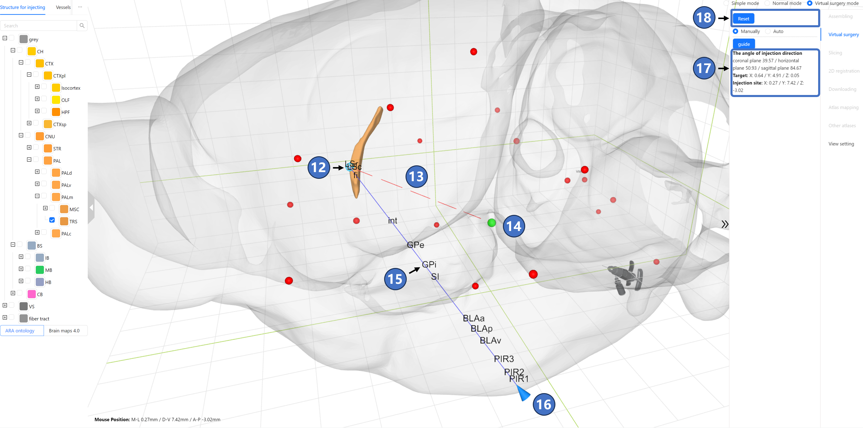
Next, select the surgery planning type. STAM offers two options: manual planning and automatic planning, corresponding to the “Manually“ and “Auto“ options in the radio button that appears as ⑪. If the user clicks “Manually“ to enter manual planning type, the marked injection target turns into a blue dot ⑫. A red dashed line ⑬ originates from the injection target and extends towards the current mouse position. The intersection of this dashed line with the outline of STAM ⑭ (i.e., the injection site) is marked in green. Once the user identifies a suitable injection path, they can left-click to mark it. The marked path will appear as a solid blue line ⑮ in the main window, with the injection site marked as a blue cone ⑯. The names of brain regions and nuclei that the path passes through will be arranged along the solid line according to their spatial positions. In the right panel, information about the angle between the injection path and three standard anatomical directions, the injection target, and the injection site is displayed ⑰. If the user wishes to restart the entire virtual surgery process, they can click the “Reset“ button ⑱ on the right panel.
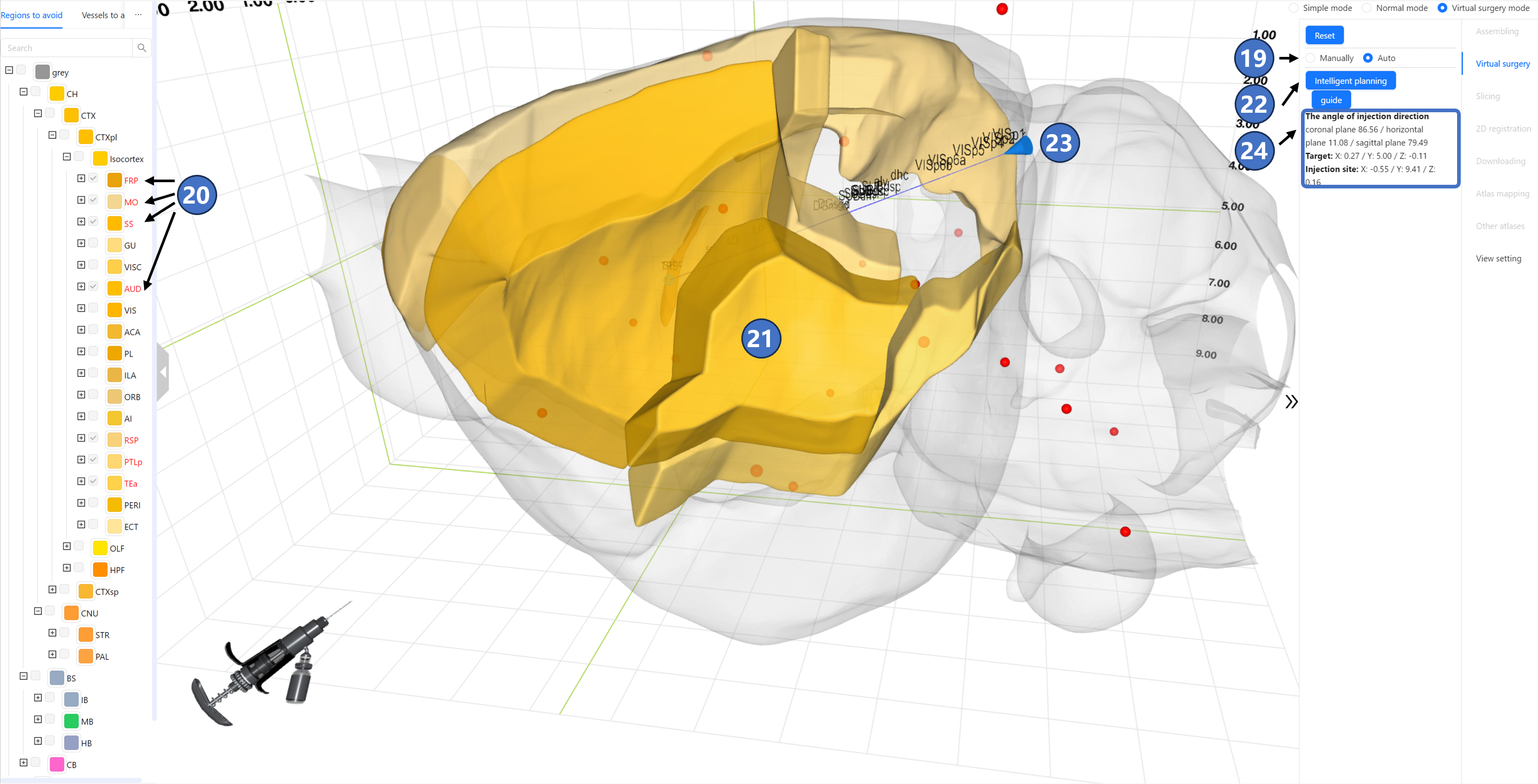
If the user clicks “Auto“ ⑲ to enter automatic type, the “Structure for injecting“ tab on the left data panel changes to “Regions to avoid“. All checkboxes besides the structures become disabled. By clicking on the names of brain regions or nuclei to avoid, the selected text will highlight in bright red ⑳. Simultaneously, the 3D contours ㉑ of these structures will be visualized in the main window. Next, clicking the “Intellectual planning“ button ㉒ on the right panel initiates the process. After a few seconds, STAM returns a path ㉓ originating from the injection target, avoiding all user-selected brain regions and nuclei. Similar to the manual planning, this path is marked as a solid blue line, with the injection site marked as a blue cone. The names of all brain regions and nuclei that the path passes through will be arranged along the path according to their spatial locations. Information about the injection angle between the injection path and three standard anatomical directions, the injection target, and the injection site will also appear on the right panel ㉔. Note that STAM's automatic planning involves a degree of randomness. If the planned path in a particular instance does not meet user’s expectation, the user can click the “Intellectual planning“ button again until achieving a satisfactory result.
Atlas reslicing
We provide services to visualize atlas reslicing from any angle. Users can choose any angle of interest and examine the isotropic 1-micron resolution 3D brain map at that angle. This service provides newly generated slices with annotations for brain regions and nuclei. The interface for the atlas mapping service is illustrated below. On the left of the main window is the data panel, which has the same function as the data panel in “Stereotaxic topography visualization”. The central area is the main window. As shown by ①, users can control the atlas reslicing's translation along the X (M-L), Y (D-V), and Z (A-P) axes by left-clicking and dragging the red, green, and blue arrows, respectively. When an arrow is selected, it will be highlighted as bright yellow. As indicated by ②, users can switch from translation mode to rotation mode by pressing the “R“ key on the keyboard.
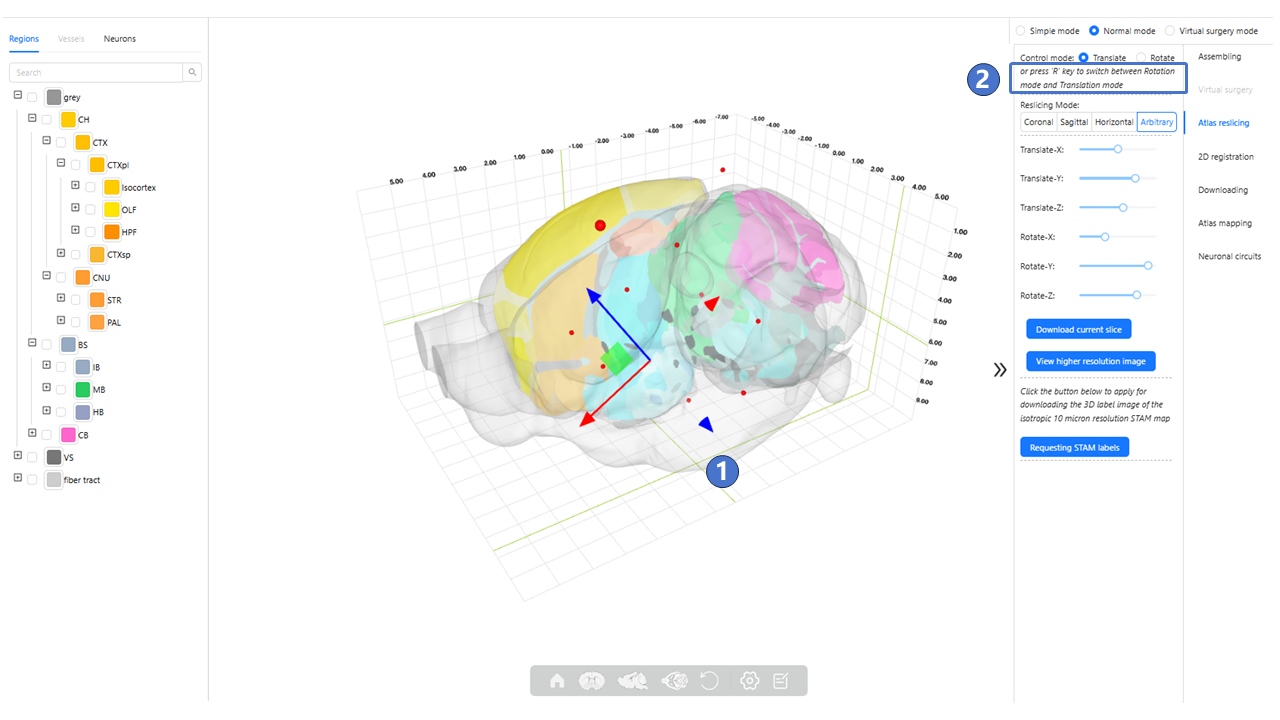
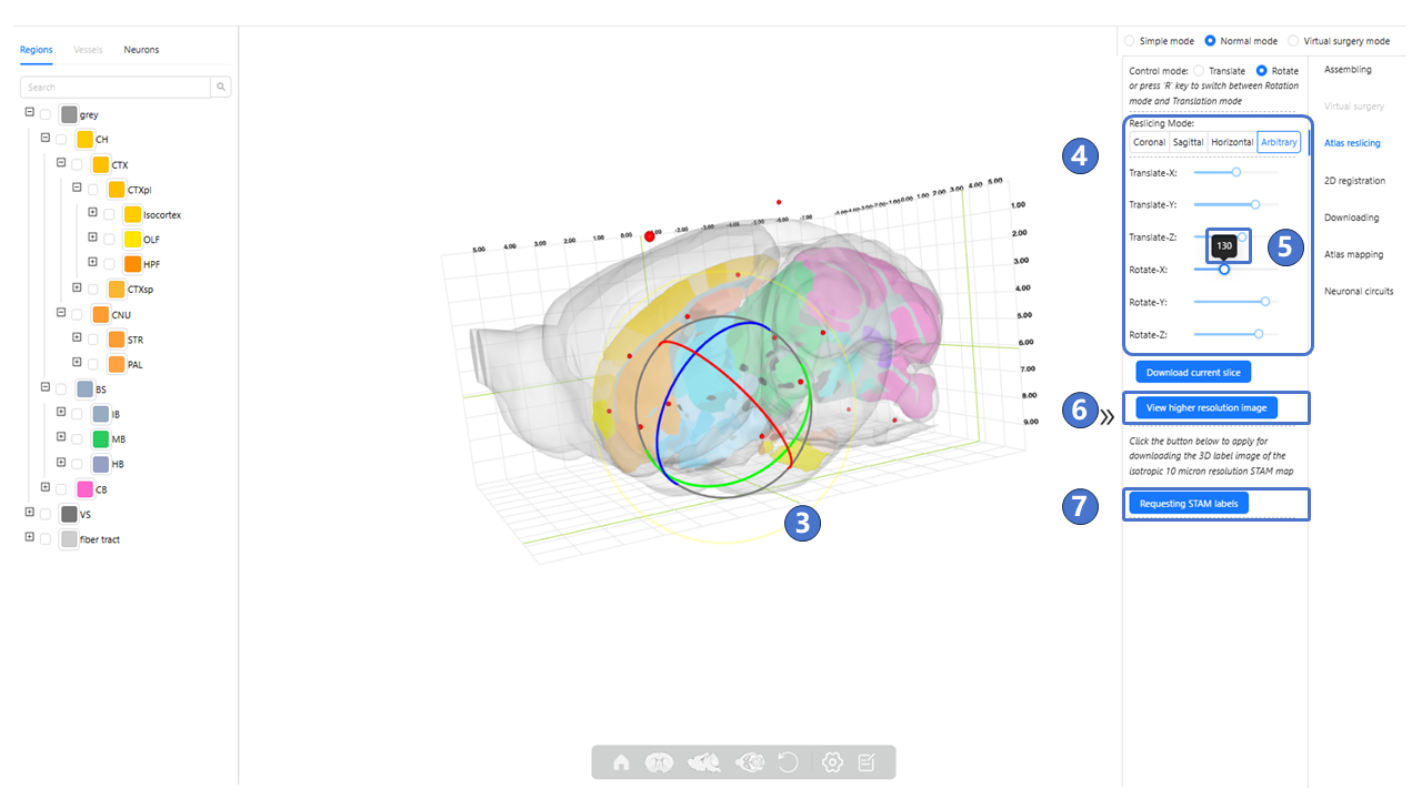
As shown by ③, in this mode, the arrows will change to sphere, and dragging these spheres will control the rotation of the atlas reslicing in the X (M-L), Y (D-V), Z (A-P) axes. Additionally, as shown by ④, users can also achieve translation and rotation of the atlas reslicing by dragging the Translate-X, Translate-Y, Translate-Z, Rotate-X, Rotate-Y, and Rotate-Z sliders ; The specific translation and rotation values can be seen in the black-background tip above the slider⑤. As shown in ⑥, clicking “viewer higher resolution image” button can jump to “Arbitrary Plane Visualization”. As shown in ⑦, clicking the “Requesting STAM labels” button will invoke the user registration page. After filling in basic information and submitting a registration request to the STAM website, the user can obtain a license. By filling in the license, the 3D label image of the isotropic 10-μm resolution STAM can be downloaded.
Neuronal circuits
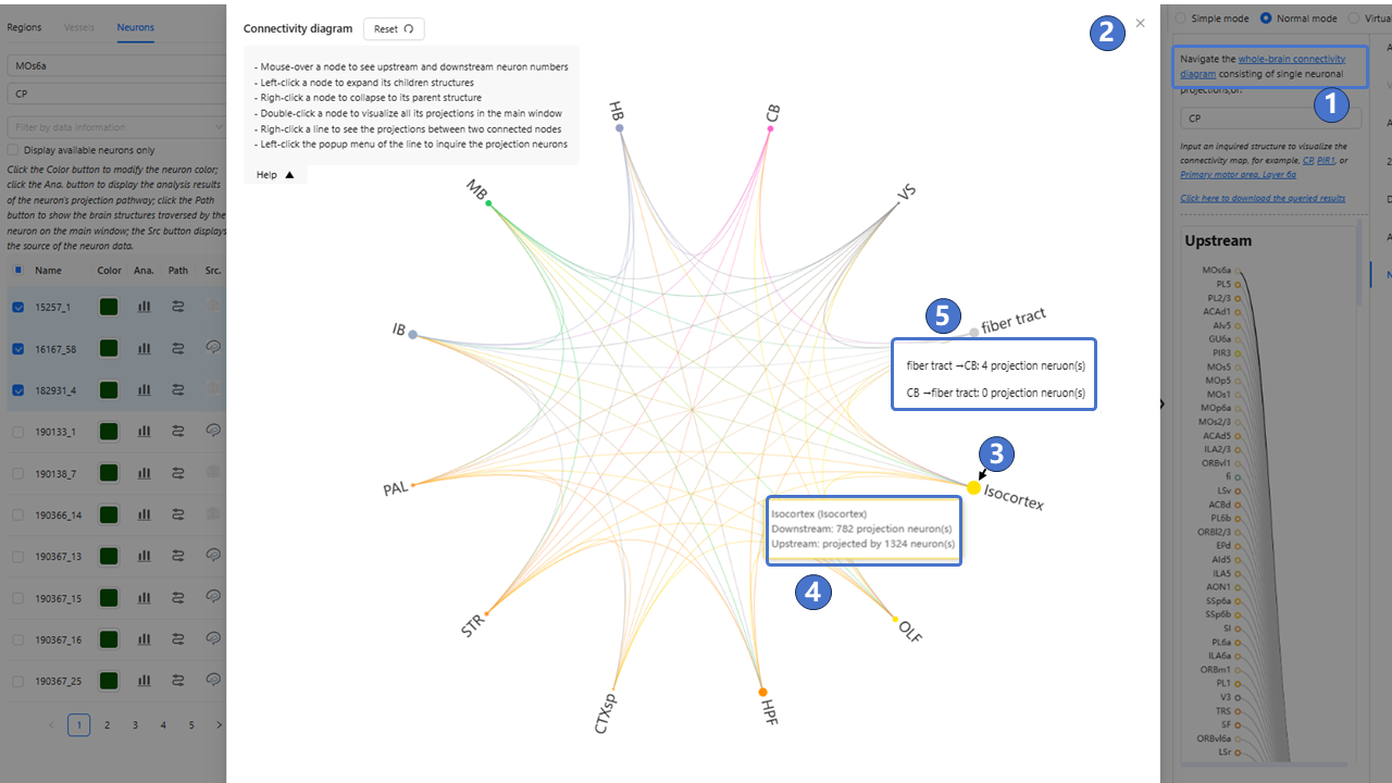
We provide services to visualize neuronal circuits of whole mouse brain somas or projection targets. Users can select any neural circuit data with somas or projection targets located in brain region or nuclei of interest, and examine the corresponding brain region and nuclei annotations of the neural circuit. The interface for the neural circuits service is shown in the figure below. On the left of the main window is the data panel, which has the same function as “ Stereotaxic topography visualization“. The “Neurons“ tab is used to query and filter neuron morphological data with somas or projection targets located in regions of interest. As shown in ①, users can click the “whole brain connectivity diagram“ button or search for the brain region or nucleus of interest in the search box to pop-up connectivity diagram composed of brain region or nuclei sub-structures②. As shown in③, different circle represent different brain region or nuclei, and the name of the brain region or nuclei is displayed next to the circle. When the user hovers the mouse over circle or name, the circle switches to highlighted mode, and display the full name of brain region or nuclei, while counting the number of upstream and downstream neurons in the brain region or nuclei④; Left-click the circle, then the connectivity diagram will display all sub-structures brain region or nuclei corresponding to the circle, as well as brain region or nuclei structures at the same level as the clicked nucleus, and show the neuronal circuits between all sub-structures; Right-click the circle to return to the previous level connectivity diagram. As shown in ⑤, when the user right-click on the connection line between brain region or nuclei, then count the number of neurons between the brain regions or nuclei, and display it on the interface.
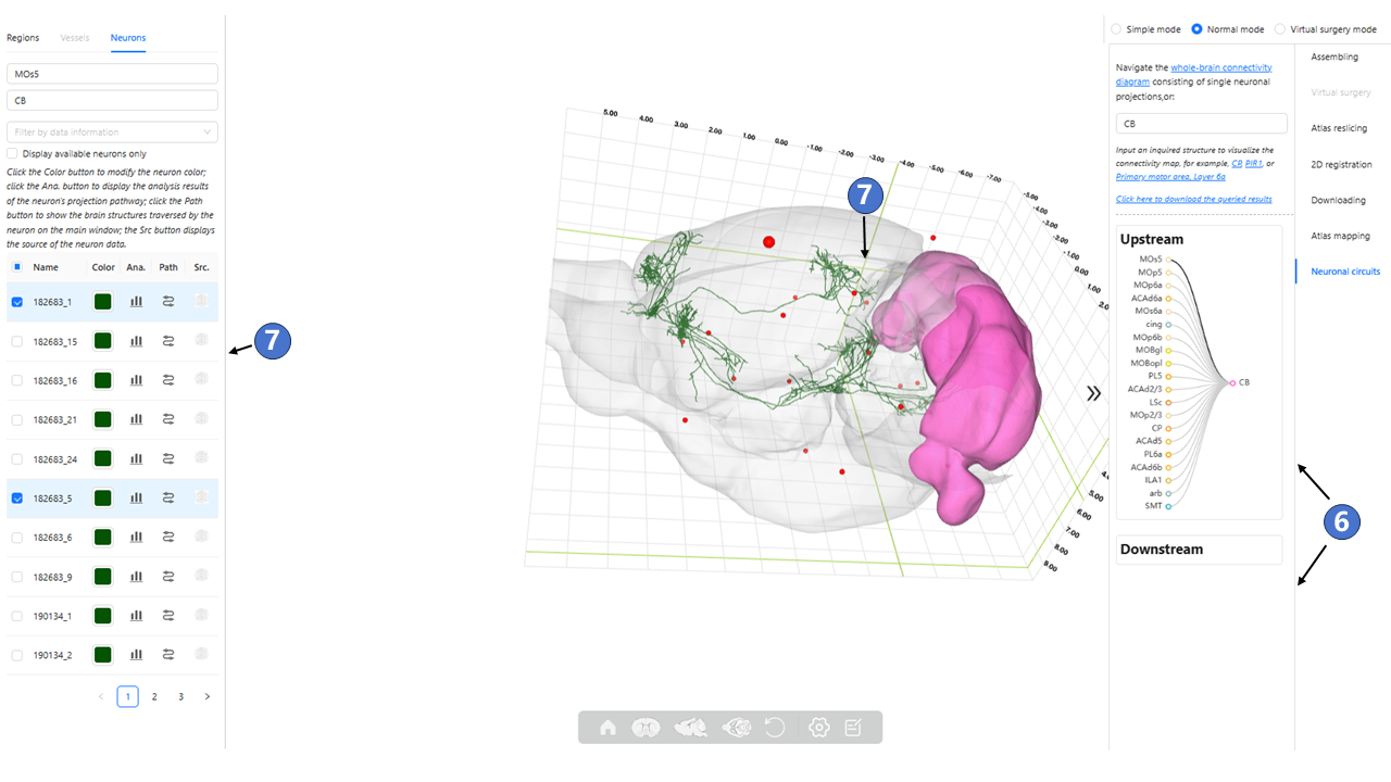
Double click on the circle to close the neural circuit connection diagram window and show the neuron circuit in the main window. As shown in ⑥, the Upstream window shows the selected somas located in brain region or nuclei of interest, and shows the projection targets in the Downstream window; As shown in ⑦, Display all neurons located in the brain region or nuclei of interest in “Neurons” tab. Users can select any number of structures of interest via checkboxes, and visualize them in the main window.
FAQ
1. How to adjust the appearance of the atlas
At the bottom of both the canonical plane visualization page and the stereotaxic topography visualization page, there is a button bar. As shown in the figure below, when viewing the canonical plane visualization page, you can control the zoom either by using the mouse scroll wheel or by clicking the button labeled ①. If you want to adjust the display mode of the atlas, you can click the settings button labeled ②, where a pop-up menu will allow you to modify the style and content of the atlas. Buttons ⑤ through ⑧ correspond to the four display modes of the brain atlas: "Atlas& image", "Atlas only", "Contour&image", and "Image only".
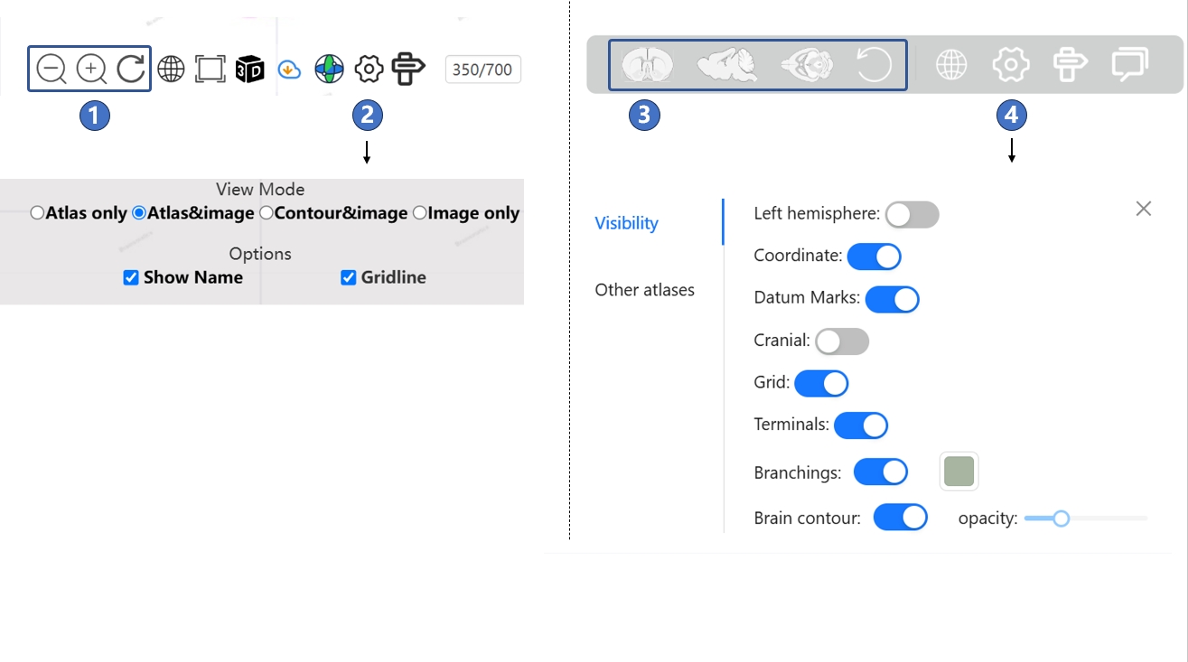
When browsing the stereotaxic topography visualization page, you can drag by holding down the left mouse button or click the button labeled ③ to adjust the viewing angle. If you want to select elements displayed in the 3D scene or modify their styles, you can click the settings button labeled ④ and make adjustments in the pop-up menu.
2. How to better observe objects of interest in 3D space by setting a focus?
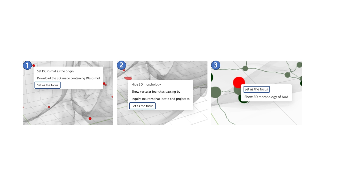
In the 3D scene of STAM, the default focus is set to the center of the brain’s outer contour. When you hold and drag the left mouse button, the view of the 3D scene rotates around this default focus as the mouse moves. This default setting is usually sufficient for standard 3D browsing needs. However, when you want to observe structures located at the edges of the 3D scene, or fine targets such as neuron branching points, you can set these objects as the new focus by right-clicking on them. Objects that can currently be set as a focus include the datum marks of STAM, the center points of anatomical structures, and the terminals or branching points of neurons, as shown in ① - ③. To recover to the default focus, you can click the reset button in the bottom button bar.
3. How to save the current 3D scene
If you have configured a 3D scene to your preference through a series of complex operations on the 3D visualization page and want to save it for future use, you can simply copy the link from your browser's address bar and save it locally on your computer. The next time you paste this link into your browser, you can directly access the previous 3D scene. In the future, we plan to develop a user system for STAM’s visualization service, allowing you to save 3D scenes of interest in your personal profile.
4. Can I change the color of visualized objects?
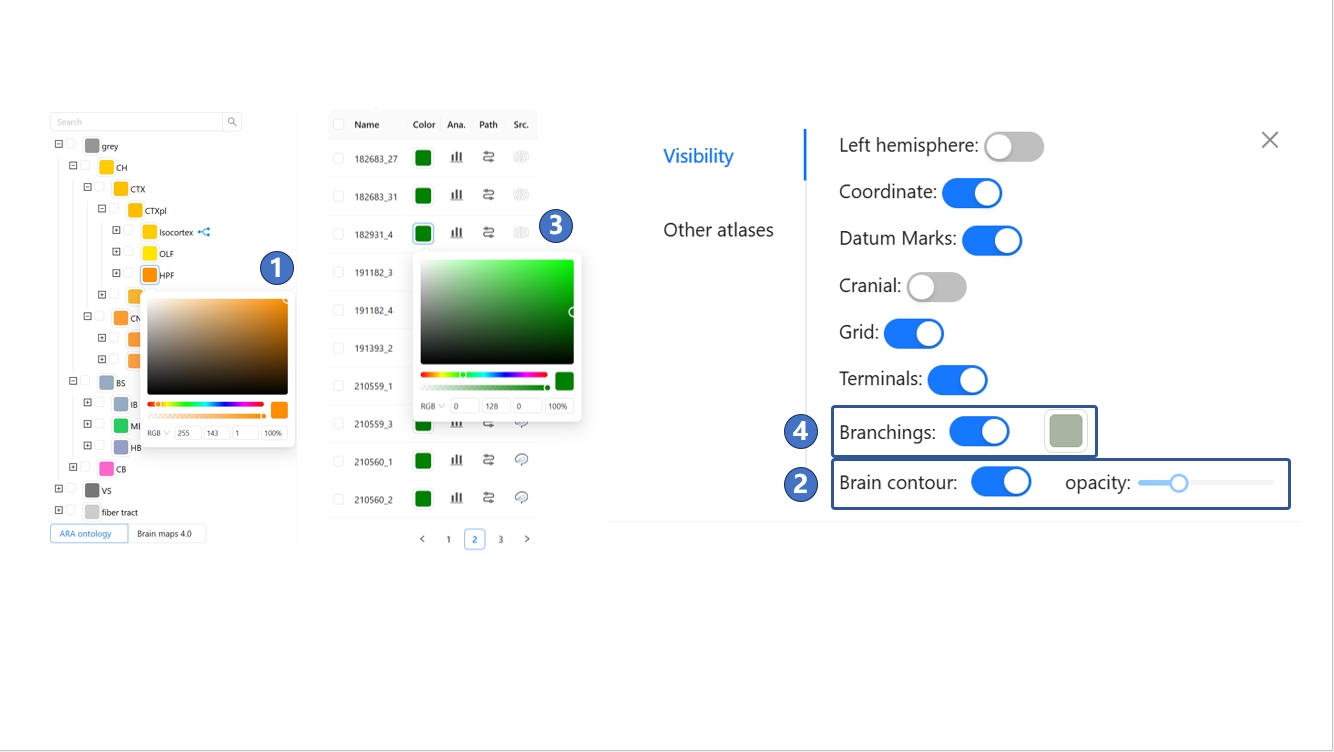
Yes, most objects in the 3D visualization scene can be customized. For anatomical structures, you can click the color block beside the text in the hierarchical ontology tree on the left side of the page, then modify its color in the pop-up interaction box, as shown in ①. For the brain's outer contour, you can click the settings button at the bottom of the interface and adjust the contour’s transparency in the pop-up panel, as shown in (2). For neurons, you can click the color block beside the text in the neuron list on the left side of the interface to change the color of the neuron terminals in the pop-up interaction box, as shown in (3). Then, you can click the settings button at the bottom of the interface and set the color of branch points in the pop-up panel, as shown in (4). The branch point color setting applies to all visualized neurons throughout the scene.
5. How to interact with higher-order brain regions
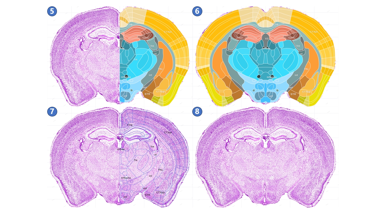
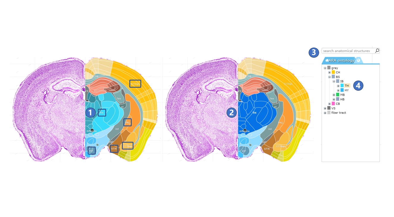
The boundaries displayed on the canonical plane visualization page represent the finest level of brain anatomical structures. However, we also provide ways to interact with higher-order brain regions. Users can click on the label text of a higher-order brain region on the page using the left mouse button, as shown in ①. This label text will be highlighted, along with all the annotations of the finest-level structures within that brain region, as shown in ②. Users can also search for the brain region, as shown in ③, or click on the name of the region in the brain anatomy hierarchical ontology on the left side of the page, as shown in ④.
6. How to interact with neurons in the 3D scene?
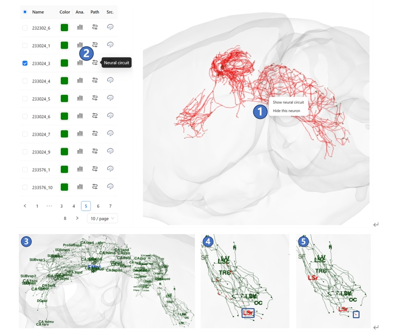
We have registered neuron morphology data from various sources into STAM's 3D space, creating a neuronal circuit database at the single-neuron level. Records that match your filter criteria will appear on the left side of the page. You can select any neuron to visualize it in the main window, then right-click on it and select the "Show neural circuit" button in the pop-up menu, as shown in ①. Alternatively, you can directly click the "Neural circuit" button on the neuron record on the left side, as shown in ②. At this point, the names of brain structures where the neuron's projection terminals and branching points are located in will appear in the 3D space, as shown in ③. You can then hover over a brain structure name, which will highlight the name text as well as the branching points and terminals within that structure, as shown in ④. You can also hover over any branching points or terminals, which will highlight both the point and the name of the corresponding brain structure it is located in, as shown in ⑤.
7. How to view quantitative analysis results of neurons?
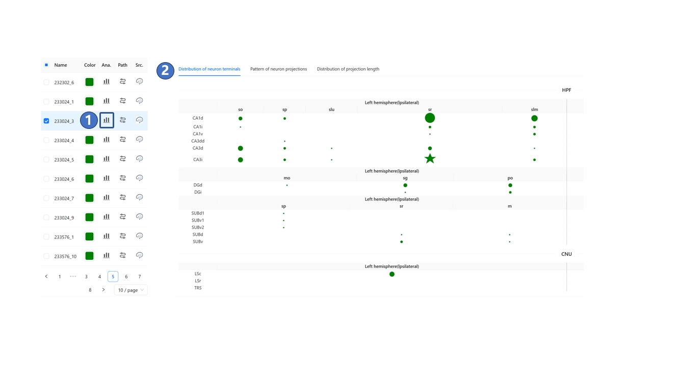
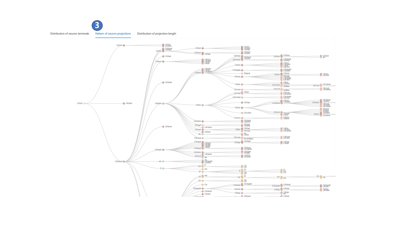
We have registered neuron morphology data from various sources into STAM's 3D space, creating a neuronal circuit database at the single-neuron level. Records that match your filter criteria will appear on the left side of the page. You can click the "Analysis" button on a filtered neuron record, as shown in ①, and in the pop-up menu, browse the distribution of its terminals, its projection pattern, and the distribution of projection lengths across different brain structures, as shown in ② and ③.
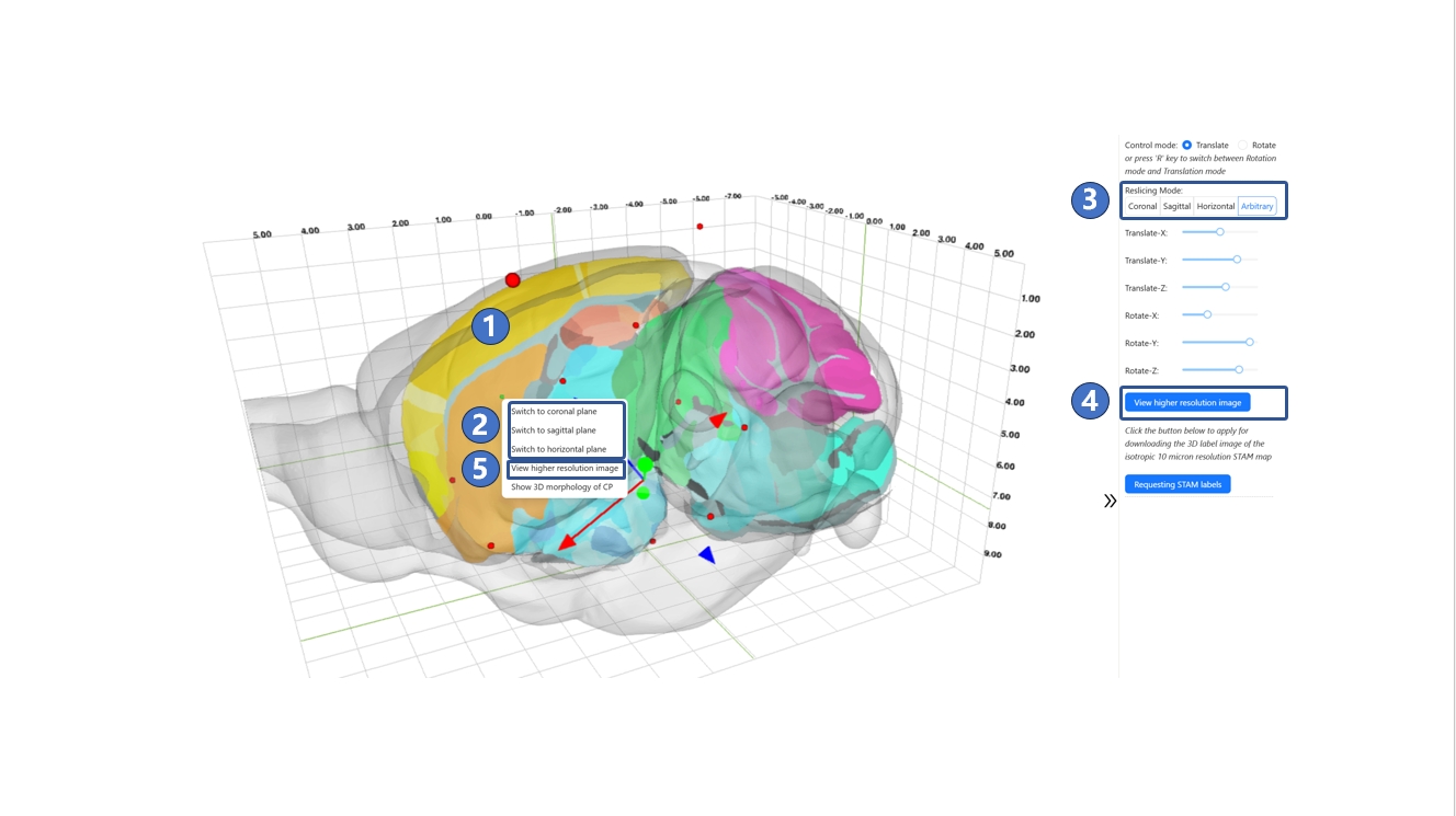
8. How to use the atlas reslicing module?
We developed the atlas reslicing module as a central hub connecting various other STAM functionalities. Through this module, you can jump to the canonical plane visualization page, arbitrary plane visualization page, or visualize the 3D morphology of any brain structure of interest directly on this page. The core of this module is a slice widget within the brain's contour, as shown in ①. By default, this slice is in arbitrary-angle plane mode, but you can switch to canonical plane mode, such as the coronal plane, as needed via the right-click menu or the control panel on the right side of the page, as shown in ② and ③. After determining the reslicing direction and adjusting the position and angle parameters, you can access high-resolution images through the "View higher resolution image" button in either the control panel or the right-click menu, as shown in ④ and ⑤. This will take you to the canonical plane visualization or arbitrary plane visualization services to view the corresponding high-resolution original images.